Cyclical Statistical Forecasts and Anomalies – Part 5

Many of you will have read the previous posts in this series and may even have a few detections running on your data using statistics or even the DensityFunction algorithm. While these techniques can be really helpful for detecting outliers in simple datasets, they don’t always meet the needs of more complex data.

In this blog we are going to look at some techniques for how we can scale anomaly detection to run across thousands of servers or users across different time periods.

What’s My Range Again?

One key concept we are going to be exploring in this blog is cardinality, that is the number of subsets or groups within our original data. This may seem like a complicated idea, so we’ll try to explain it with some simple examples. Taking the previous blog posts in this series, the main factor when considering cardinality is time: for example, we were looking at splitting our data into daily and hourly groups in parts 1 and 4 of this series, which makes a cardinality of 24x7=168. 

Often splitting data by time alone is not enough for anomaly detection, for example if you are trying to baseline user behaviour then you might want to split out your anomaly detection models by time and user. So, if you are running an anomaly detection analytic in an organisation with 1000 users with different behaviours depending on the time of day and day of week then the cardinality is much higher: 24x7x1000=168,000.

At this level of cardinality, the approaches outlined in the previous blogs will either: struggle to complete the calculations or produce giant lookups (which may have secondary effects on your Splunk instance such as destabilising kv store processes). 

Therefore, it’s really important that you consider the cardinality in your data ahead of applying any anomaly detection technique! Although it’s not a perfect rule, generally if your cardinality is over 1000 then using the DensityFunction isn’t optimal, and if it creeps above 100,000 then using a statistics-based approach isn’t optimal.

Handling Data with High Cardinality

Knowing that datasets with a cardinality above a hundred thousand can cause issues with some of the typical methods for applying anomaly detection, we're going to describe a few techniques for reducing cardinality.

Here we’re going to cover how you can use Principal Component Analysis (PCA) to reduce the dimensions in your data and another approach using Perlich aggregations to describe the likelihood of values occurring in your data. 

Note: that we will be using a dataset that ships with the MLTK in this blog, and although the dataset has pretty low cardinality it is a useful set for showcasing the techniques.

Principal Component Analysis

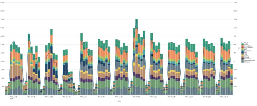
PCA is a way of compressing a set of input variables down into a lower dimensional set of variables, all while maintaining the overall behaviour of the input variables. Using PCA is something that has been employed with good effect by companies like Netflix to detect outliers in high cardinality data as described here. When it comes to applying PCA in Splunk there is a simple example below, where we are using PCA to reduce our 11 inputs into a single dimension.

| inputlookup app_usage.csv 

| fit PCA CRM CloudDrive ERP Expenses HR1 HR2 ITOps OTHER Recruiting RemoteAccessWebmail k=1

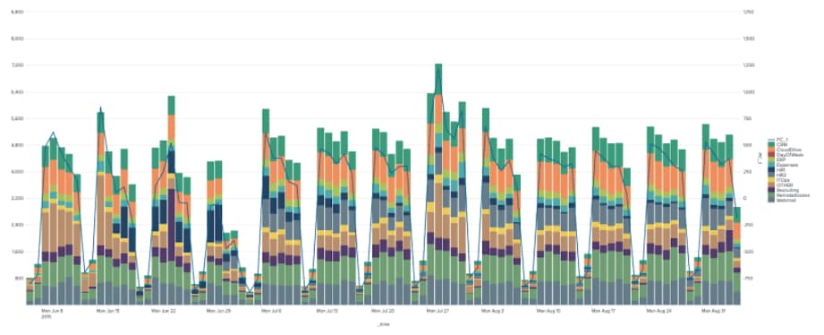Focusing now on just a single metric we can apply DensityFunction to identify outliers on a per-day basis as in the chart below.

| inputlookup app_usage.csv 

| fit PCA CRM CloudDrive ERP Expenses HR1 HR2 ITOps OTHER Recruiting RemoteAccessWebmail k=1

| eval _time=strptime(_time,"%Y-%m-%d") 

| eval DayOfWeek=strftime(_time,"%a") 

| fit DensityFunction PC_1 from DayOfWeek

As you can see from the chart PCA has helped us identify times when the overall behaviour of all the apps we are monitoring look unusual, but perhaps isn’t as sensitive to individual app behaviours.

Normalised Perlich Ratio

We’re now going to consider how we can use Perlich aggregations, which are good for converting high-cardinality fields in data into something more manageable. You can read a primer on the subject here or find a whole load more detail here. Essentially, they convert descriptive data, such as a username or a host into a ratio that describes the likelihood of that username or host occurring compared to the rest of the data. This technique will allow us to dig deeper into individual app behaviours, also creating an outlier ‘score’ that is representative of the overall set of behaviours for our applications.

For our example we are going to calculate ratios for the app name based on a discretised buckets of the variable we are looking for outliers in. In this exact case we are going to calculate a ratio that describes how likely an app is to have a certain level of events associated with it. 

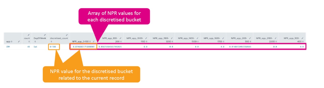
When you run the NPR algorithm in Splunk it actually returns a full array for each target and feature variable, which describes the likelihood of the feature variable occurring against the list of target variables. In reality all we care about is the current feature and target combination – i.e., the likelihood for the record in question – which is just one entry from the array as shown in the diagram below. Luckily, we can unpick the right record using the foreach command.

| inputlookup app_usage.csv

| untable _time app count

| bin bins=30 count as discretised_count

| fit NPR discretised_count from app

| foreach NPR_app_* [| eval NPR_app=if(NPR_actual="<<FIELD>>",NPR_app+'<<FIELD>>',NPR_app)]

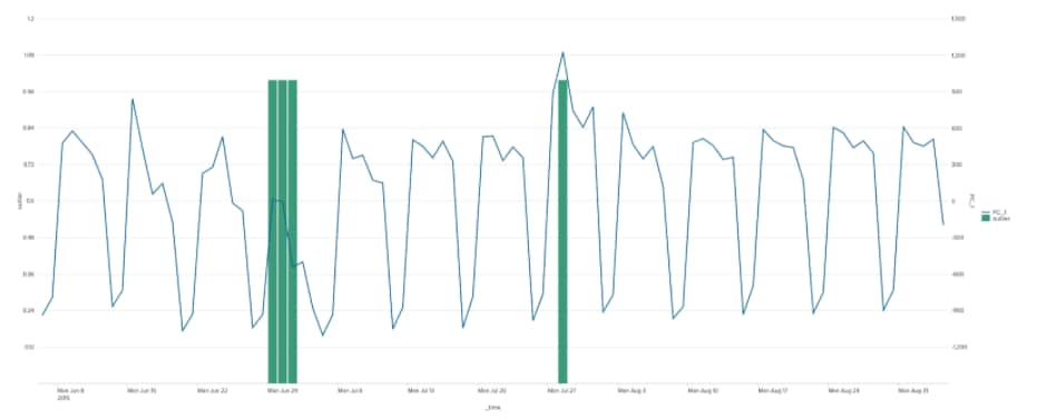
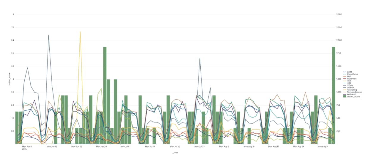
Using the calculated likelihoods, we can then flag data as anomalous if the likelihood falls below a certain value as in the chart below, where the anomaly score is the sum of all outliers for all apps at any given point in time.

| inputlookup app_usage.csv

| untable _time app count

| bin bins=30 count as discretised_count

| fit NPR discretised_count from app

| eval NPR_actual="NPR_app_".'discretised_count', NPR_app=0

| foreach NPR_app_* [| eval NPR_app=if(NPR_actual="<<FIELD>>",NPR_app+'<<FIELD>>',NPR_app)]

| eval outlier=if(NPR_app<0.01,1,0)

Alternatively, we could use another anomaly detection method using the NPR values we have calculated and the raw data itself. The example below shows how the Isolation Forest algorithm can be used against the NPR values, the count and the day of the week to identify potential outliers – again in the chart the outliers have been summed up to create an outlier score.

| inputlookup app_usage.csv

| untable _time app count

| bin bins=30 count as discretised_count

| fit NPR discretised_count from app

| eval NPR_actual="NPR_app_".'discretised_count', NPR_app=0

| foreach NPR_app_* [| eval NPR_app=if(NPR_actual="<<FIELD>>",NPR_app+'<<FIELD>>',NPR_app)]

| table _time app count NPR_app 

| eval _time=strptime(_time,"%Y-%m-%d") 

| eval DayOfWeek=strftime(_time,"%a")

| fit IsolationForest DayOfWeek count NPR_app

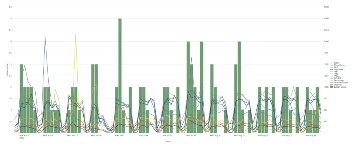With this type of ensemble method we are flagging outliers based on the likelihood of an apps behaviour being in a certain range and also using the cyclical time series information and raw count too – which provides a more holistic view on each event than just using the likelihoods.

Summary

We have now walked through a few useful techniques for identifying anomalies in datasets with high cardinality, but please note that this has not been an exhaustive overview of anomaly detection on these types of datasets! I have often seen situations where customers have needed to apply NPR, PCA, scaling algorithms and a more complex detection using a clustering algorithm such as DBSCAN.   

Now it’s over to you to see if you can find outliers in your largest datasets, and of course happy Splunking!